Optimizing AI Deployments with VMware Cloud Foundation (Part 4)

Utilizing Time-slicing to Optimize Inference Throughput

Introduction

The Broadcom Performance team has completed extensive performance tests demonstrating VCF’s efficiency and flexibility for running AI workloads in various configurations. To explain our results, we’ve published a white paper and a series of four blogs:

• Part 1: Maximizing Performance, Efficiency, and Flexibility in Multi-tenant Environment
• Part 2: Maximizing GPU Utilization for Best Total Cost of Ownership
• Part 3: Maximizing CPU and Memory Utilization for Best Total Cost of Ownership
• Part 4 (this blog post): Utilizing Time-Slicing to Optimize Inference Throughput

Today we are happy to share with you part 4 of this series.

---

This blog explores how NVIDIA vGPU on VMware Cloud Foundation (VCF) optimizes GPU utilization by using time-slicing. Unlike traditional partitioning, this approach allows virtualized workloads to, in some cases, outperform bare-metal configurations by intelligently sharing compute resources.

Time-Sliced vGPU vs. Multi-Instance GPU (MIG) 

There are two primary ways to share GPU resources in a virtualized environment. Both approaches isolate memory. They differ on the axis that determines everything: whether compute cores are partitioned or scheduled. 

	Time-Sliced vGPU	Multi-Instance GPU (MIG)
High bandwidth memory	Statically partitioned, strictly isolated	Statically partitioned, strictly isolated
Compute cores	Time-sliced, round robin across VMs	Statically partitioned into hard instances
Peak compute per workload	Full GPU while it holds its time-slice	Capped at its partition – always
Neighbor’s idle cycles	Scheduler reallocates unused slices	Idle cycles stranded in partition
Starvation risk	None – every VM has a guaranteed minimum	None – boundaries are fixed in hardware

Why this matters: MIG vGPU’s rigid boundaries prevent one workload from using another’s spare capacity. vGPU’s round-robin scheduler still guarantees each VM a minimum allotment, but lets it exceed that allotment whenever a neighbor skips its turn. 

The “Time-Slicing” Advantage:

Strategy	Resource Allocation	Result
Layout A (Traditional) – See Figure 1	Uses three vGPUs on three physical GPUs	Standard performance based on three-GPU compute
Layout B (Optimal) – See Figure 1	Spreads the same memory requirement over four physical GPUs	Accesses compute cores from all four GPUs, significantly increasing throughput

The core innovation lies in spreading a workload’s vGPU profiles across more physical GPUs than strictly necessary for its memory requirements. The workload then absorbs compute cycles its neighbors leave idle — beating bare metal on aggregate throughput (our testing showed 30% better than bare metal on models from Hugging-Face, 10% better than bare metal for models compiled with TRT-LLM). The gain scales with slack; the less optimized the model, the more idle cycles exist to reclaim.

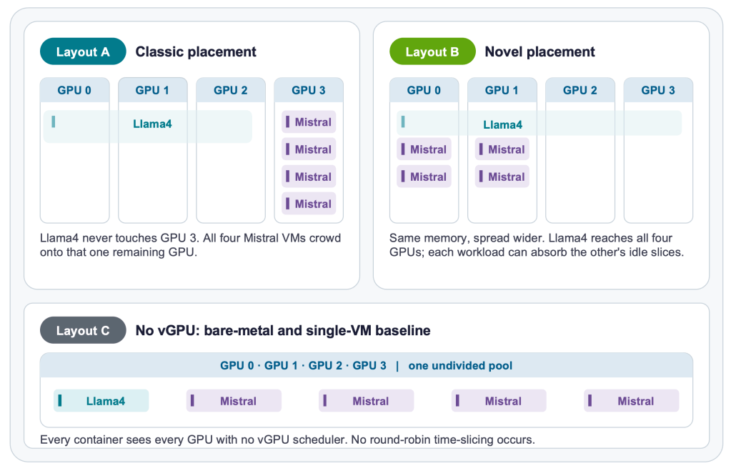
Figure 1: Three different placements of the workloads: 1x Llama4 17B, and 4x Mistral 7B. 

The classic placement (“Layout A”) has a total of five VMs: one running Llama4 17B and four VMs running Mistral 7B. The Llama4 17B model uses three physical GPUs and the Mistral models share the fourth GPU. 

The novel placement (“Layout B”) exploits time-slicing. In Layout B, the Llama4 17B spreads its vGPUs over all four physical GPUs, and the Mistral workload spreads over the two physical GPUs that have GPU memory available. If all four GPUs had GPU memory available, we could have spread the Mistral over all four GPUs. Layout B allows a workload to use compute cycles that are not being used by another workload on the same GPU. This results in higher aggregate throughput than with Layout A. Since NVIDIA vGPU on VCF uses time-slices that are assigned round-robin to the VMs, no workload will be starved of compute resources. Every workload is guaranteed a minimum compute allotment, but can receive more if another workload is not using its time slice. 

The third placement (“Layout C”) has only one VM on ESX (or runs without VMs on bare metal). Layout C assigns all four NVIDIA A100-80C GPUs to every container; i.e., the containers share the GPUs. Layout C does not support pre-emption, so a workload that uses only one GPU could starve a workload that needs all the GPUs. In addition to being unfair, it also leaves plenty of GPU compute unused.

Layout B allows a workload to claim as much GPU compute as possible while only reserving the minimum GPU memory necessary. It is particularly effective for embarrassingly parallel workloads, such as:

• LLM Inference: e.g., Llama 3/4, Mistral.
• Financial Analytics: High-performance computing (HPC) tasks, such as “computing the Greeks.”

Where the extra throughput comes from: A single GPU’s compute cycles, before and after the change in VM-to-GPU assignment. Nothing is added to the machine; previously stranded capacity simply becomes reachable. 

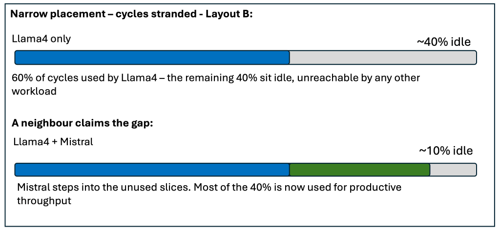
Figure 2: A conceptual illustration of round-robin slice reallocation. This is not measured data.

How the scheduler behaves:

• Slices are handed to VMs round-robin, so no workload is ever starved. Each keeps a guaranteed minimum compute allotment. 
• When Llama4 is between batches and skips its turn, Mistral runs in that window instead of the GPU sitting idle. 
• The effect compounds across every GPU on which a workload has a profile, which is why spreading profiles wider raises aggregate throughput. 

The caveat that bounds the whole result: A workload tuned to saturate every available cycle leaves nothing behind for a neighbor. That means the time-slicing advantage disappears entirely when there are no idle cycles to reclaim.

Experiment 1: Unoptimized Workloads (Hugging Face)

One Llama4 17B and four Mistral 7B instances running concurrently on a PowerEdge XE8545 with two AMD EPYC processors and four NVIDIA A100-80 GPUs. 

Configuration	Layout	Time-Slicing	Result
Multi-VM, 5 VMs on vGPU	B	Yes	130 – Highest
Bare metal, containers in Ubuntu	C	No	100 – Baseline

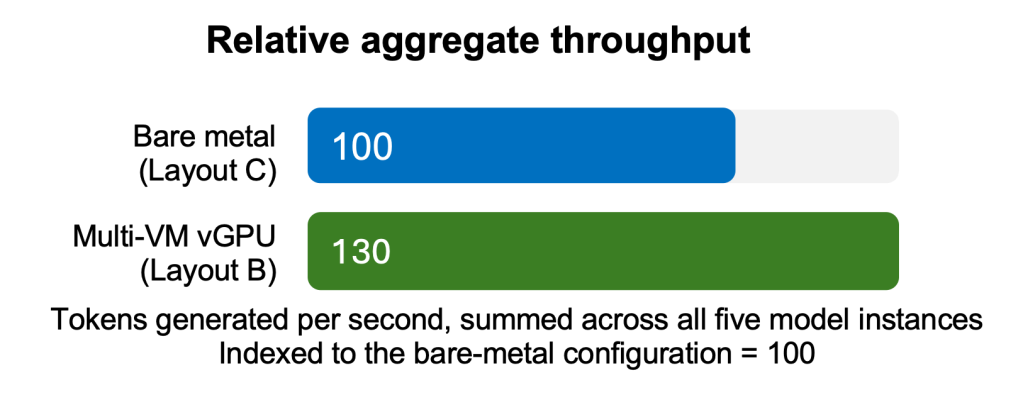
Figure 3: The normalized relative aggregate throughput. Bare metal is indexed to 100 and is the baseline.

Takeaway: All three configurations use identical hardware. The 30% delta comes purely from letting the vGPU scheduler redistribute the compute cycles that Layout C leaves idle. 

Experiment 2: Optimized Workloads (NVIDIA TensorRT-LLM)

Llama3 70B in fp16, compiled with TensorRT-LLM and run across the same four A100-80 GPUs under three different tensor and pipeline-parallelism settings. 

Configuration	Parallelism	GPUs	Result
2 VM, one instance each	PP=2(PP = Pipeline Parallelism)	2 per VM	110 – Highest
Bare metal, one instance	TP=2, PP=2 (TP = Tensor Parallelism)	4	100 – Best bare metal

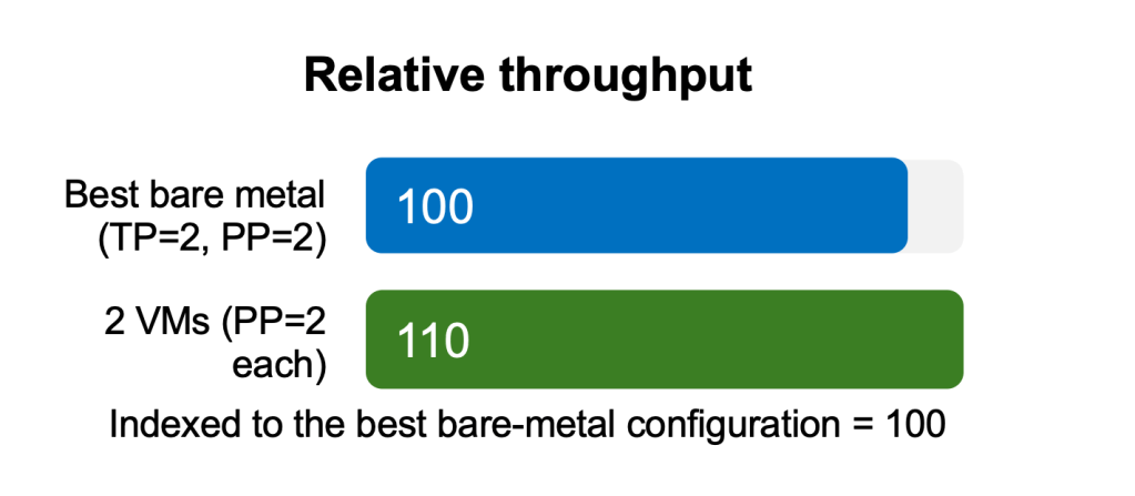
Figure 4: The normalized relative aggregate throughput. Bare metal is indexed to 100 and is the baseline.

Why the gain shrank from 30% → 10%: TensorRT-LLM compilation removes most of the slack that time-slicing feeds on. Fewer idle cycles remain, so there’s less for a neighboring VM to reclaim. The mechanism is unchanged; its fuel supply is smaller. 

Conclusion

By leveraging the time-slicing capabilities supported by VCF, organizations can achieve higher aggregate inference throughput compared to standard non-time-sliced configurations. The magnitude of this throughput improvement is inversely related to the level of optimization of the workload. Lightly optimized workloads — such as raw models pulled directly from Hugging Face — can see performance gains of up to 30%, whereas heavily optimized models running via TensorRT-LLM will often see lower, though still notable, improvements in the range of 10%. 

We recommend fully optimizing your models first, then leveraging strategic workload placement to unlock the maximum performance benefits of vGPU time-slicing.