

Columnar storage earned its place in analytics for a simple reason: when a query only needs three columns out of thirty, you shouldn’t have to pay the computation and memory costs for the other twenty-seven. Append-Optimized Columnar (AOCO) tables in VMware Tanzu Greenplum have delivered on that promise for years. But “scan only the columns you need” is only half the efficiency story. The other half is “scan only the rows you need.”
In part one of this two-part series, we explore how Tanzu Greenplum 7.6 tackled this hurdle by introducing Implied Index (also known as the Ghost Index), a feature that accelerates selective WHERE-clause queries on AOCO tables without the storage or maintenance overhead of secondary indexes.
Tanzu Greenplum’s AO Columnar Store is already designed for efficient, high-speed analytics by eliminating the need for storage-intensive indexes and their ongoing maintenance. The Implied Index builds on this foundation with:
- Direct row identification: pinpoints matching rows in columnar data, minimizing unnecessary reads
- Selective materialization: surfaces only the rows that satisfy query predicates, conserving resources
- Cross-column bitmap filtering: combines filters across columns to efficiently handle multi-column conditions
The result is an index-free architecture purpose-built for analytical workloads with selective WHERE clauses: delivering fast, scalable performance while keeping operational complexity and storage costs low.
The problem with the old paths
Before this optimization, querying a columnar table meant choosing between two imperfect strategies:
- Column projection scans: the engine reads every value in the required columns in full, stitches rows back together, and then applies the WHERE clause filter. This works well for broad aggregations, but it means you pay the full I/O and decompression cost even for rows that get thrown away moments later.
- Traditional index lookups: a secondary index gets you directly to matching tuple IDs, avoiding wasted reads, but at a price. Indexes consume extra storage, slow down ingestion and updates, and don’t generalize well. Indexes also do not support compression, even when the base table is compressed. In other words, the same column ends up inflating the index far more than it did stored in the table. A table queried sometimes by severity and sometimes by location needs an index on each, and every filter combination you didn’t anticipate falls back to a full scan anyway.
Neither approach lets you have cheap, targeted access to arbitrary filter combinations without ongoing index maintenance overhead. Here’s what that tension looks like on an actual table.
Example
Picture an events table stored as AOCO, with columns like event_name, event_time, event_type, severity, and location, each physically stored as its own contiguous column with a ctid (row identifier) alongside it:
SELECT event_name FROM events WHERE event_type IN ('Cyber Incident');

- With column projection, the engine reads
event_nameandevent_typein full for every row, stitches the two columns together byctid, and only then discards rows whereevent_typeisn’t'Cyber Incident'. Every non-matching row’sevent_namestill got read and stitched for nothing. - With a traditional index on
event_type, the engine does an index lookup to get the matchingctidsfirst, then fetches only the correspondingevent_namevalues. But now imagine the next query filters onseverity = 'Critical', orlocation = 'Acme Security Agency'instead. Without an index on those columns too, you’re back to a full scan. Indexing every column that might show up in aWHEREclause defeats the purpose of columnar storage in the first place.
The idea: Treat the columnar store itself as the index
Implied Indexing’s insight is that a columnar store already has most of what an index provides. The values are stored contiguously per column, in a highly compressed fashion that helps reduce I/O for reads, with positional metadata connecting them back to rows. So instead of building a separate structure, Greenplum 7.6 changes how the scan executes:
- Qual-first scanning: only the columns actually referenced in the
WHEREclause are scanned in full first, not the entire projection list. In the example above, that means readingevent_typein full but leavingevent_nameuntouched for now. - Tuple identification: matching row IDs are identified directly from that initial, narrow scan.
- Multi-column filter evaluation: AND conditions are checked sequentially with immediate short-circuiting when a filter fails, producing the final matching row IDs.
- Selective materialization: the engine fetches and materializes the remaining projected columns (
event_name) only for the rows that survived the filter.
The net effect is that non-matching row data for the wide, expensive columns (the ones not in the WHERE clause) is never pulled off disk or decompressed at all. The filter column effectively becomes the index, hence the name Implied Index. And because it’s derived from the column itself rather than a separate structure, it adapts to whatever filter the query happens to use. For example, severity today, location tomorrow. This is done without the end user having to pre-build an index for either.
It’s a cost-based decision, not a blanket rule
Locating the right rows this way, however, isn’t entirely free. It carries a small amount of overhead of its own. What Implied Indexing saves is skipping disk I/O for data that contains no matching rows and skipping CPU work for rows that won’t appear in the result set. For the optimization to pay off, those savings need to outweigh its own overhead, so the query optimizer makes this call on a cost basis: Implied Indexing is only chosen when it’s actually cheaper than a plain sequential scan.
How much it actually helps: the experimental data
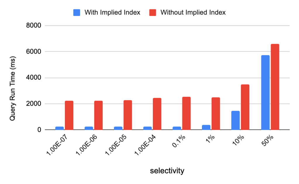
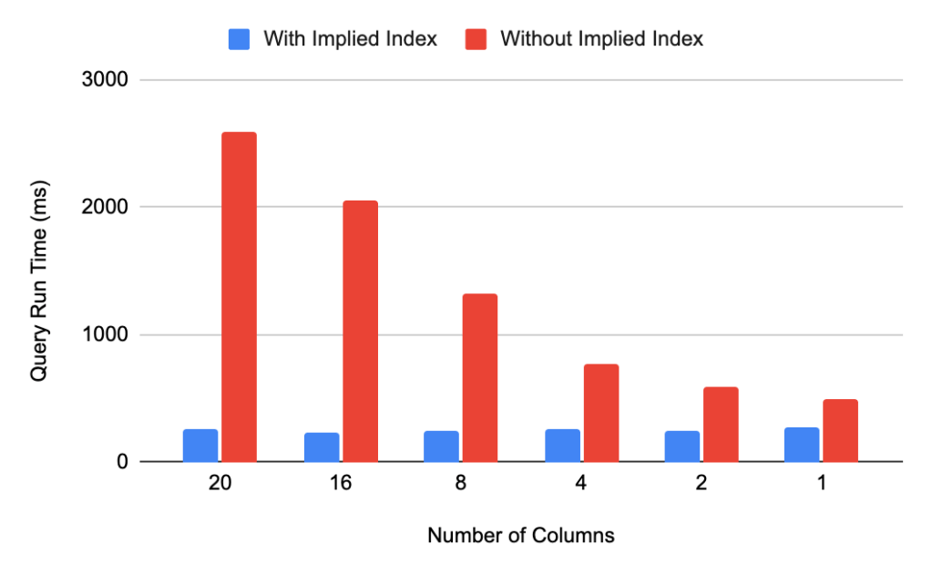
That cost-benefit line isn’t just theoretical; it shows up clearly once you measure it. Three factors dominate how much Implied Indexing gains, tested on a 10-million-row, 20-integer-column AOCO table (uncompressed, warm cache):
1. Selectivity: fewer matching rows means bigger wins. At very high selectivity (a predicate matching roughly 1 row in 10 million), Implied Indexing ran ~10x faster than a plain scan. As selectivity drops, more rows match and the benefits of filtering decrease. That is, the gain shrinks to about 1.15x at 50% selectivity, the point where the block directory overhead starts eating into the savings and the optimizer may stop choosing this path at all.
2. Target list size: more projected columns means bigger wins. With a highly selective predicate, projecting all 20 columns showed a ~10x speedup, since every one of those 20 columns benefits from not being materialized for discarded rows. Projecting just a single column narrowed that to about 1.8x. There’s simply less unnecessary work left to eliminate when the target list is already small.
3. Qual size behaves differently depending on the operator. For predicates chained with OR (disjunctions), where each individual qual is already highly selective on its own, adding more OR‘d columns steadily erodes the gain. It drops from ~10x with a single predicate down to about 1.15x with 16. That’s because every additional ORed column must be scanned regardless of whether earlier ones matched. For predicates chained with AND (conjunctions), the story is much better: even with 16 columns in the qual, Implied Indexing still delivered roughly a 2.5x speedup (versus ~10x with just one). That’s because AND evaluation can short-circuit: once an earlier qual fails for a row, the engine skips checking the remaining qual columns for that row entirely, so qual size ends up mattering far less than selectivity or target list size.
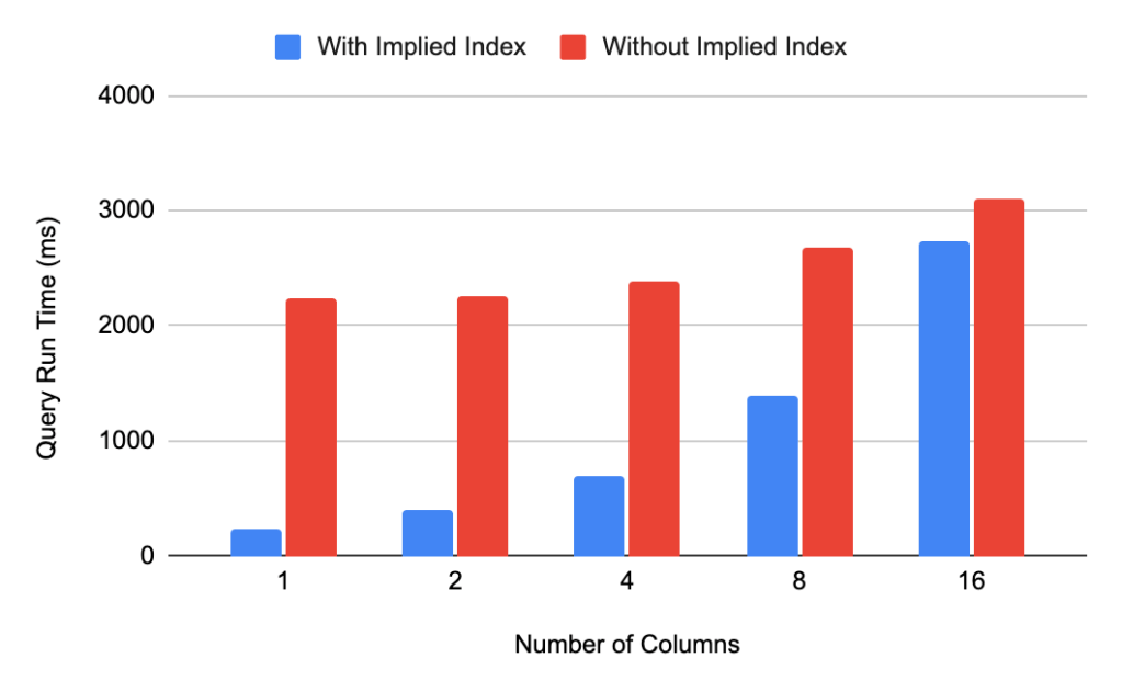
Figure 4. Effects of number disjunctive predicates (OR)
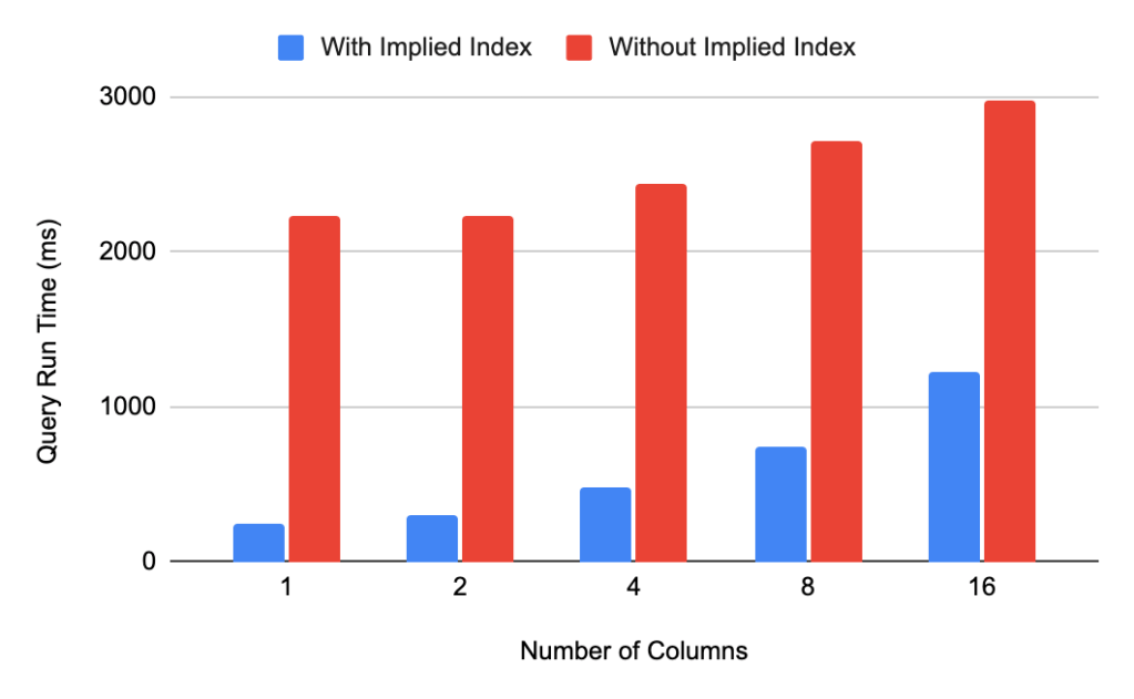
Figure 5. Effects of number conjunctive predicates (AND)
In Summary
Implied Indexing resolves the classic columnar tradeoff: full-scan I/O costs versus the storage and maintenance overhead of indexes. By treating the columnar store itself as the index, Tanzu Greenplum 7.6 delivers targeted, index-like access to any filter combination, without requiring a single index to be built or maintained.
The gains are largest exactly where columnar workloads need them most: selective predicates, wide projection lists, and AND-heavy filters, with speedups up to 10x. Because the optimizer applies this on a cost basis, it only activates when it’s actually beneficial, so there’s no downside on low-selectivity queries.
The result: faster analytics by default, with one less indexing decision for teams to make.
In part two of this series, we will explore how Tanzu Greenplum 7.9 tackles this exact bottleneck with Early Join Filtering (EJF), bringing the same “read less, decide early” efficiency directly into complex join operations.
Read part 2 of this blog series on optimizing columnar storage: Accelerating Hash Joins with Early Join Filtering
