Application and Network Admins need to be able to identify, understand, and react to changes in operational conditions of their cloud applications and data center operations. Any changes to operational conditions might be critical as they may be a reflection of business risk. On the flip side, some of these deviations could be precursors of positive growth.
Detecting abnormality is therefore essential and may offer interesting business insights. Consider these scenarios:
- A cloud provider wants to know any infrastructure changes such as resource failures or excessive ingress/egress network traffic.
- The information security team wants to know abnormal user login patterns.
- A retail company wants to know events/discounts which actually trigger spikes in product purchase.
Identifying anomalies in all such cases requires building behavioral models that can automatically learn and correct the criteria for differentiating between the normal and the abnormal. A behavioral model represents (not surprisingly) the behavior of the data. A well constructed model can not only help identify outliers, but can also facilitate predictive analysis. Note that a simple approach of using static thresholds and alerts is impractical for the following reasons:
- Scale of the operational parameters: There are more than a thousand network, infrastructure, and application metrics that are required for analyzing operations of a cloud application.
- Too many false positives or negatives: If the thresholds are tight there can be too many false positives. If they are too relaxed real abnormalities could be missed.
To address operational constraints in the above scenarios, we have added another behavioral learning technique to our arsenal; an algorithm for identifying outliers in seasonal time series data.
Enter Holt-Winters Algorithm
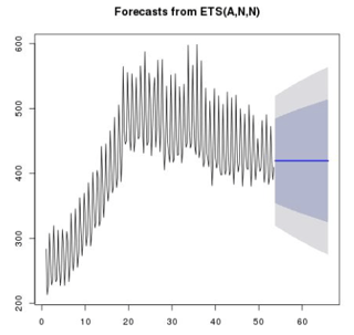
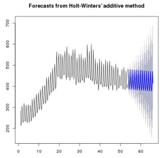
Holt-Winters (HW) algorithm, devised by Holt and Winters, helps build a model for a seasonal time series. This technique improves upon Avi’s existing outlier detection paraphernalia, which uses the Exponential Weighted Moving Average(EWMA) algorithm. If EWMA sounds greek, the following textbook Forecasting: Principles and Practice is a good quick refresher. In essence, EWMA follows the data curve closely, however, it is limited by the fact that periodic components of the data are simply ignored. This contrasts with the Holt-Winters decomposition of a signal. For a comparison between the prediction models of the two algorithms, consider the 80% and 95% prediction intervals of EWMA and HW when applied to the same data:


It is evident that ignoring seasonality of the input series can be unforgiving.
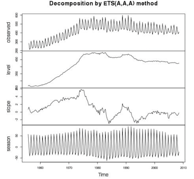
The HW algorithm works by breaking the said time series into three components:
- Level: Think of this as the intercept of a line.
- Trend: Represents the slope or the general direction of movement of data.
- Season: Highlights the periodicity of the data
The figure below presents the three ingredients of the time series we forecasted above (plotted using R):

A time series can have additive/multiplicative trend/seasonality. For the simplicity of this article, we assume application of HW to a time series with additive-trend-additive-seasonality (HW-AA). For such a series, the trend and seasonal components increase linearly, and combine additively, to compose data points at progressive time instants. The time series is represented as:

where the individual components update themselves as shown here:

Note that each component equation is essentially an EWMA-style update. For further reading, please refer to Forecasting: Principles and Practice.
A quick word about the smoothing parameters alpha, beta, gamma. As a general guideline, we employ the following equation to determine the smoothing parameters, as motivated in Aberrant Behavior Detection in Time Series For Network Monitoring

The equation highlights how much weight we want to give to historical data. For instance, at Avi, when applying HW to the metric representing application bandwidth, we give 95% weight to (5 min) samples in the last hour. Plugging these values in the above equation:

This intuition applies to other smoothing parameters. Note that as evident from update equations above, the memory footprint of the HW algorithm is proportional to the seasonal period. In context of Avi’s Analytics Engine, this implies a footprint of the size of 96KB per metric. Therefore, of the thousand odd metrics that Avi analyzes, we carefully balance application of HW to most relevant (seasonal) metrics without burdening operations.
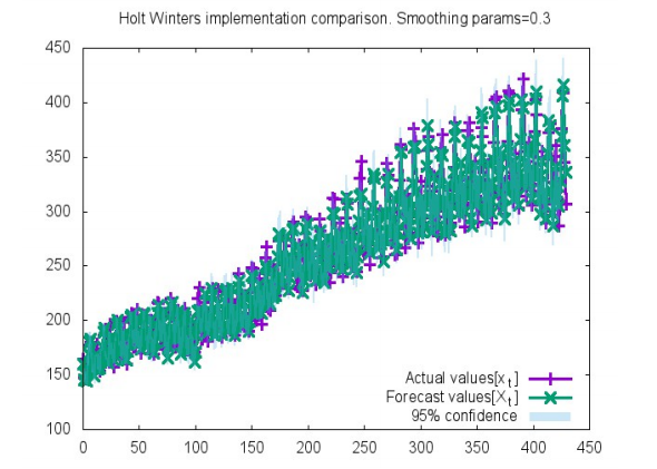
To evaluate our choice of parameters for our inline implementation of the HW algorithm, we compare the forecasted values against a known time series. Here’s the cake:

The X-axis represents the time instant, t, and the Y-axis represents the corresponding data sample value. The graph is a comparison between the original and the forecasted values, and also outlines the prediction intervals with 95% confidence. It is easy to observe that the original and forecast data aligns well.
Avi’s Analytics Engine applies multiple anomaly detection techniques to a single time series. As described above, the detection techniques employ EWMA and HW variants. Thus, the outcomes from each model are subject to consolidation modes of ALL/ANY, wherein, either all outcomes must agree on the decision (of labelling the data point as anomalous) or any would do. The choice of the consolidation mode is influenced by the tradeoff between sample false positives and true postives. In a ANY consolidation, higher false positives with higher true positives are expected as diagnosis by even one model is enough to flag a data sample as anomalous. On the contrary, the ALL mode requires a unanimous decision, which requires a greater confidence in labeling a data sample. Consequently, this makes it harder to flag legitimate data as anomalous (thus lower false positives and lower true positives). Within our product, we preset modes depending on the metric.
Conclusions
We have presented here, the Holt-Winters analysis over a time series of metrics that characterize a data center. The algorithm accounts for seasonality in data and thus, is able to better detect outliers while giving accurate forecasts for periodic data patterns.
Here are advantages of Avi’s approach:
- It is inline: – It is an intrinsic feature of the Application Delivery Controller (ADC) and does not require any additional setting or software integration.
- It is fast and actionable: The anomaly detection is performed in real-time and several mitigations actions are inbuilt into the operations. Admins do not have to manually block offending clients, or start a new server, or increase capacity based on the resource utilization predictions, etc.
- It is intelligent: Machine learning of operational patterns and behavior allows Avi’s Analytics Engine to make better decisions on detection of outliers, prediction of load, elastic capacity planning etc.
As noted earlier, we may use the model for outlier identification, and also for predicting outcomes in the future. In fact, the prediction models are used by Avi Analytics Engine for autoscaling resources. This requires capacity estimation which can have a diurnal or other seasonal pattern. Thus, the predicted capacity can now be used to spin up/down application instances, significantly optimizing cost for our customers.
At Avi, we are constantly improving our technology by developing and incorporating smarter techniques. In addition to integrating Holt-Winters into our anomaly detection machine, we are developing models that capitalize on machine learning and deep learning theories. The input from such new concepts and technologies continues to provide high quality actionable intelligence and reinforce the value of Avi Networks to our customers.


